References:

• S.N.MathTutorials

• EasyMathWithIbrahim

• Daffodil International University, BD (https://elearn.daffodilvarsity.edu.bd/course/view.php?id=6323#)

• [Initial Value Problem, IVP]https://resources.saylor.org/wwwresources/archived/site/wp-content/uploads/2011/04/DIFFERENTIAL-EQUATIONS-AND-INITIAL-VALUE-PROBLEMS.pdf\

• Dr. Gajendra Purohit

• UC Function: https://razorjr.files.wordpress.com/2010/05/methodundeterminedcoeff.pdf

• National Open University of Nigeria (Math Book) https://nou.edu.ng/coursewarecontent/MTH232.pdf

• Blackpenredpen

• TheOrganicChemistryTutor

• Udvash Engineering Concept Book

• Wikipedia

• Byjus

• CUEMATH

Integration Formulae and tricks

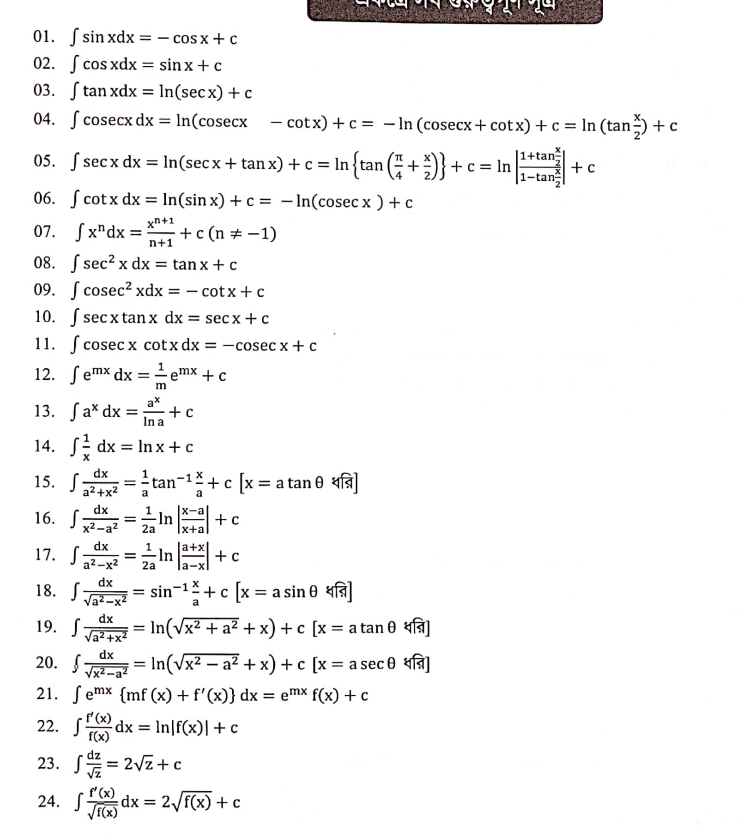
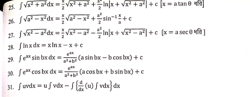
Credit: Udvash Engineering Concept Book

All Formulae: https://elearn.daffodilvarsity.edu.bd/pluginfile.php/578401/mod_resource/content/4/Formula of Differentiation and integration.pdf

Definition of Differential :

• involving derivatives of one or more dependent variable w.r.t one or more independent variable

Dependent/Independent Variable:

${\frac{dy}{dx}}$

x = independent

y= dependent (y depends on x, y is a function of x)

Types :

• Ordinary Diff. : If independent variable is one

• Partial Diff : If independent variables are > one

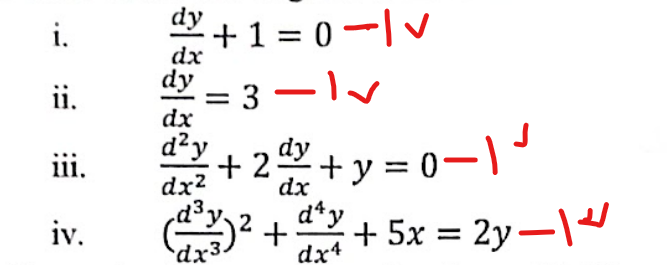
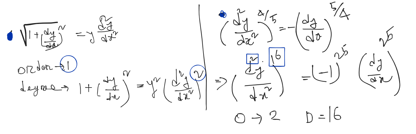
Order:

• Highest order derivative

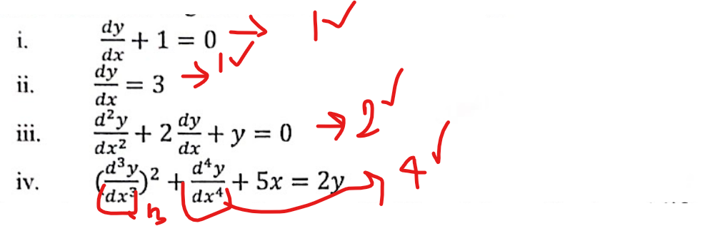
Degree:

• Highest order derivative’s power

• Degree can’t be fractional, so if there’s any fractional variable or derivatives (not only the highest derivative, it is applicable for all variables) we need to make it integer first.

→ How ? → Squaring, cubing…^n-ing the whole equation

Problems:

NB: Don’t define degree if ${\frac{1}{y}} {\frac{dy}{dx}}, {\frac{\frac{dy^2}{dx^2}}{\frac{dy}{dx}}}$, first make it like multiple of $y$, $\frac{dy}{dx}$ for the example.

Transcendental Function:

Definition: In mathematics, when a function is not expressible in terms of a finite combination of algebraic operation of addition, subtraction, division, or multiplication raising to a power and extracting a root…

Keywords: function which are return a infinite series

• If any derivative locates like this sin(derivative function), cos(derivative function), e^(derivative function), then the degree will be undefined.

Example:

1) $e^{\frac{dy}{dx}} = 5y$

Order : 1

Degree : Undefined

2) $sin(\frac{dy}{dx} ) {\frac{d^2y}{dx^2}} + 6y = 0$

Order : 2

Degree : Not defined

3) $siny + \frac{d^3y}{dx^3} = 22$

Order : 3

Degree : 1 (No derivative function in the $sine$)

Wronskian Theorem:

Let $y{_1}(x)$ and $y{_2}(x)$ are two solution of second order linear differential equation then Wronskian of $y{_1}, y{_2}$ is

$W(y{_1},y{_2}) = \begin{vmatrix} y{_1} & y{_2} \\ y'{_1} & y'{_2} \end{vmatrix} = y{_1}y'{_2} - y'{_1}y{_2}$

$W(y{_1},y{_2}) == 0$ → Linearly Dependent Solution

$W(y{_1},y{_2}) \not= 0$ → Linearly Independent Solution

If there’re $y{_1},...., y{_n}$, then the equation will be like below

$W(y{_1},...,y{_n}) = \begin{vmatrix} y{_1} & y{_2} & ... & y{_n} \\ y'{_1} & y'{_2} & ... & y'{_n} \\ ..... \\ y^{n'}{_1} & y^{n'}{_2} & ... & y^{n'}{_n} \\ \end{vmatrix}$

Linear Differential Equation:

• $({\frac{dy^n}{d^nx}})^m$ m must be 1

• There will be no $y . \frac{dy}{dx}$ , $\frac{dy}{dx} \frac{dy^2}{d^2x}$, $\frac{dy}{dx} \frac{dz}{dx}$

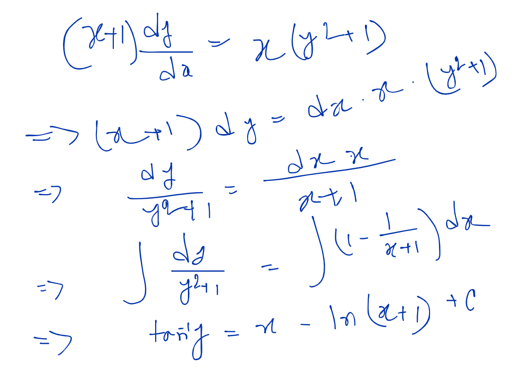
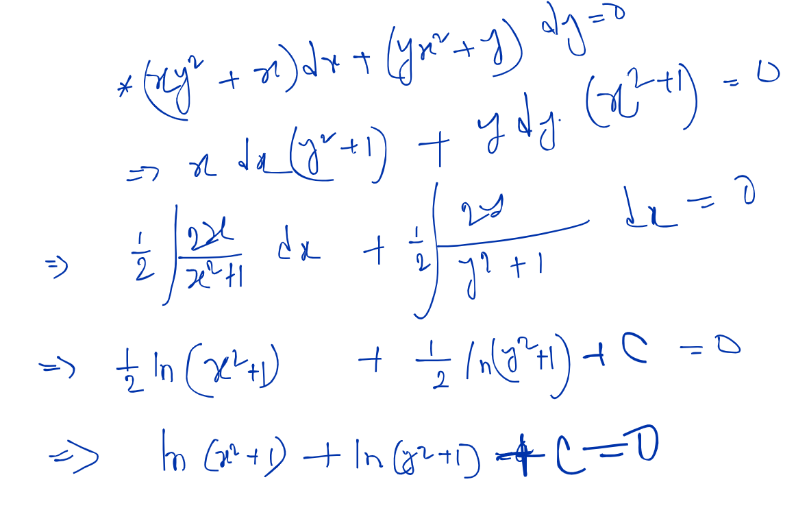
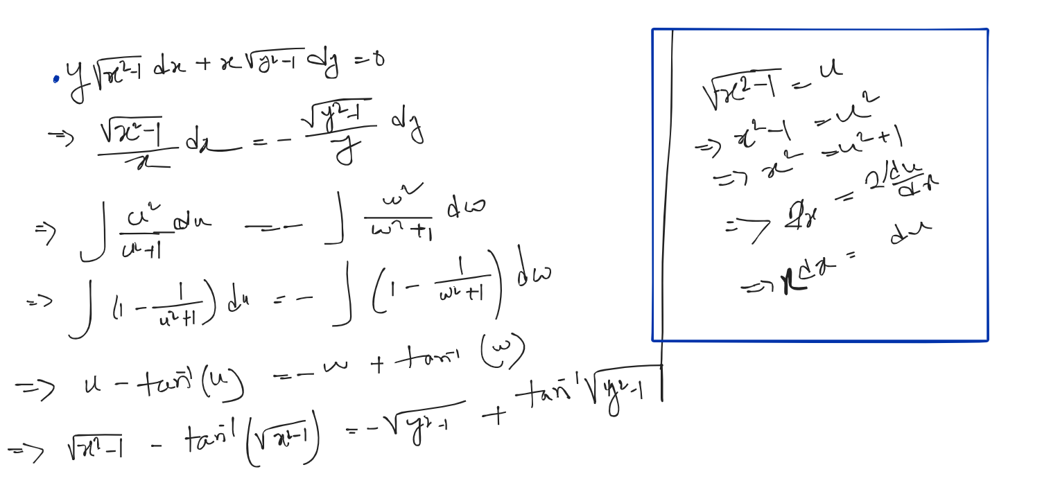
Variable Separable Method:

Steps:

• Make the equation like that f(x) = f(y)

• Integrate it

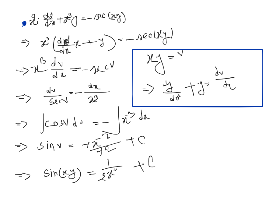
Problems:

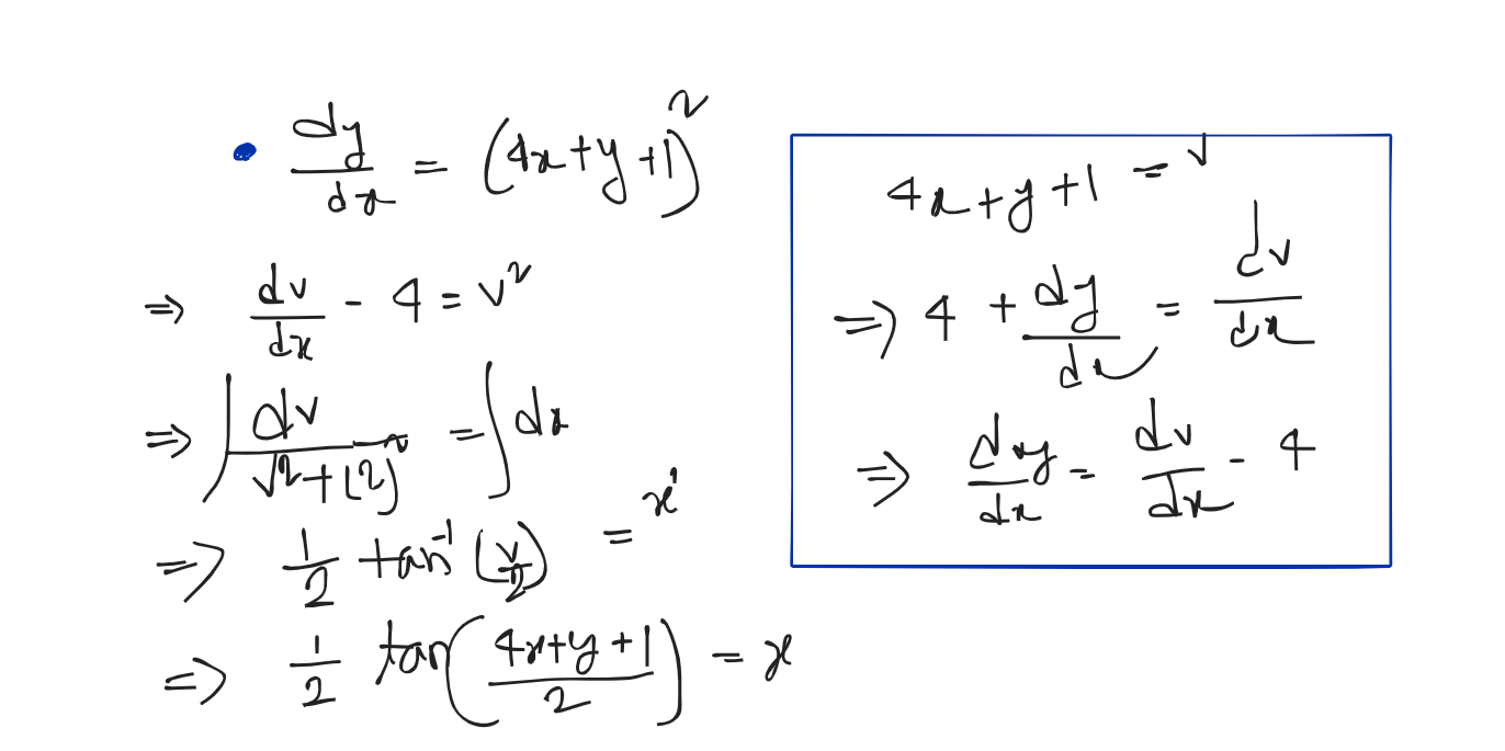
Reducible to Variable Separable Method:

If the equation like that,

$\frac{dy}{dx} = f(ax+by+c) .. .(i)$

C may be 0.

$ax + by + c = v$ or something else to solve the problem

$\frac{dy}{dx} = \frac{dv}{dx} + ....$ .. (ii)

Put $\frac{dy}{dx}$ from (ii) value in (i) and $ax + by + c = v$

Trick: term which one is repeated more than one = v

Problems:

Mistake : $xdx = udu$

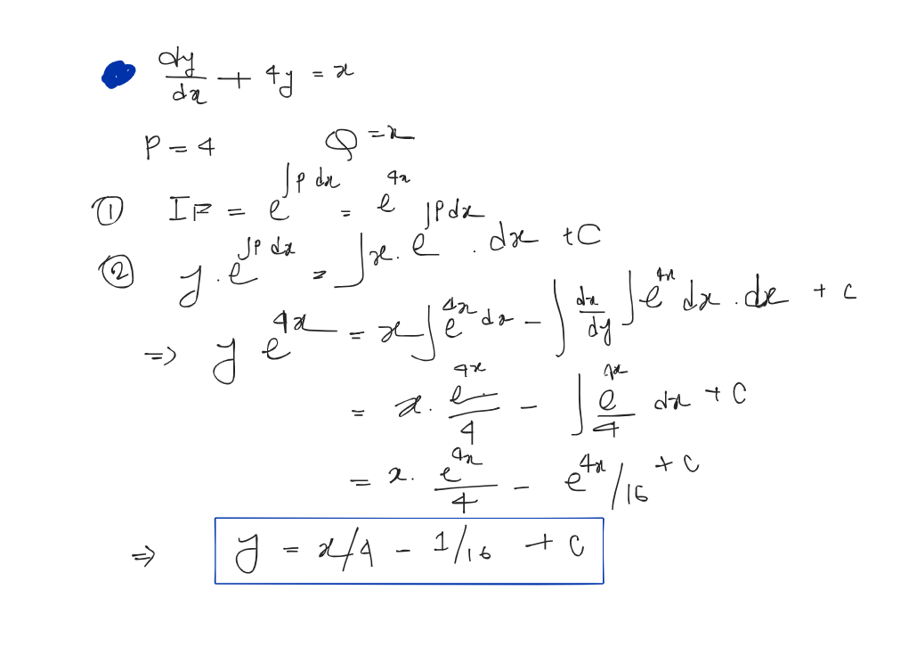
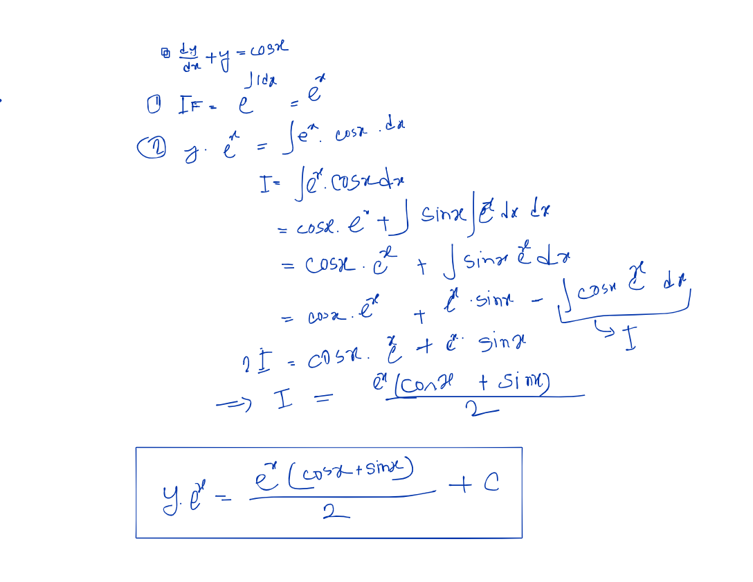
Linear Differentiation Equation:

Definition: If P and Q are only functions of x or constants then the differential equation of the form 𝑑𝑦/𝑑𝑥 +𝑃𝑦 = 𝑄 is called the first order linear differential equation.

$\frac{dy}{dx} + yP = Q$

Where P and Q are constant or function of x. Then, linear differentiable equation is applicable. Otherwise Separable Method.

Step:

• Integrating Factor $I{_f}$ = $e^{\int{Pdx}}$

A given differential equation may not be integrable as such. But it may become integrable when it is multiplied by a function. Such a function is called the integrating factor (I.F).

dx = independent variable. If y is an independent variable then, it would be Pdy.

• General Solution: and Calculate

$yI{_f} = \int{Q I{_f}dx} + C$

Problems:

Homogenous Differentiation Equation:

Definition: An equation of the form $\frac{dy}{dx} = \frac{𝑓{_1}(𝑥, 𝑦) }{𝑓{_2}(𝑥, 𝑦) }$ in which $𝑓{_1}(𝑥, 𝑦)$ and $𝑓{_2}(𝑥, 𝑦)$ are homogeneous functions of x and y of the same degree can be reduced to an equation in which variables are separable by putting $𝑦 = 𝑣𝑥$ , $\frac{dy}{dx} = v + x\frac{dv}{dx}$

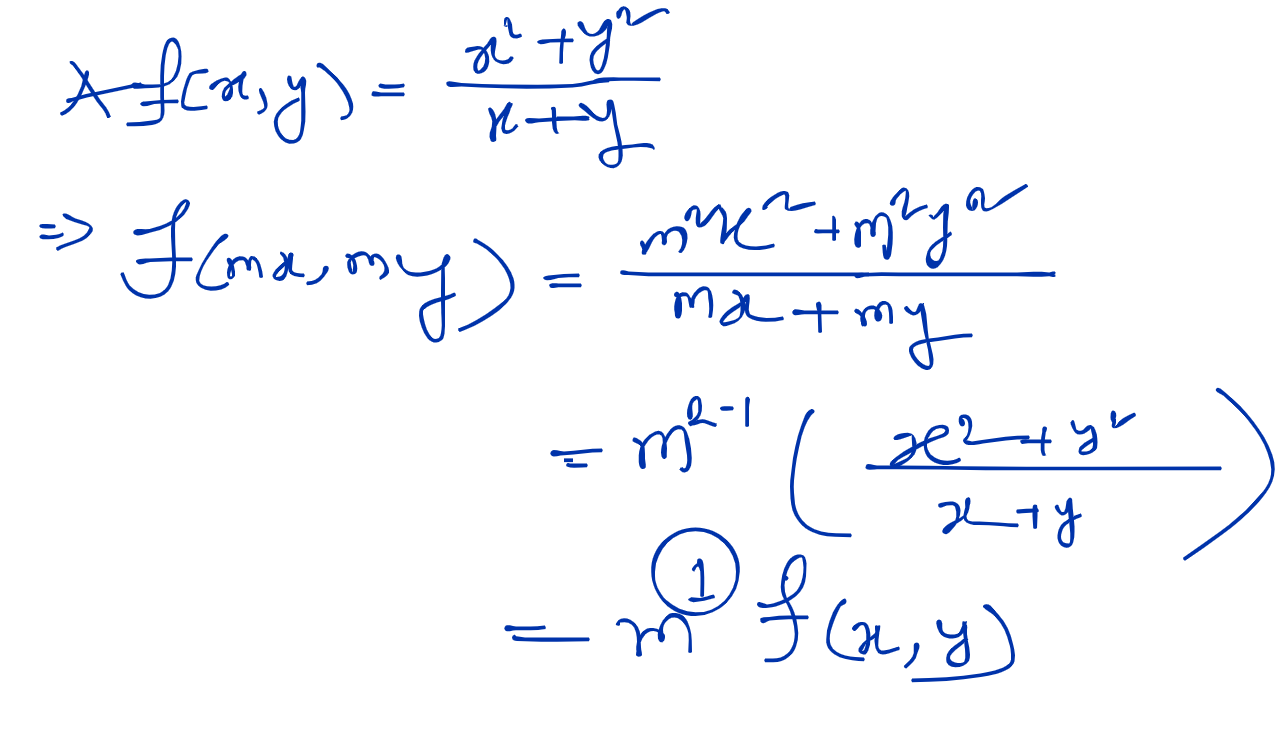
Homogenous Function & It’s Degree: $F(x,y)$ is homogenous function and $n$ is the degree of the function then if $f(mx, my) = m^n f(x,y)$, where $m$ is a non-zero value.

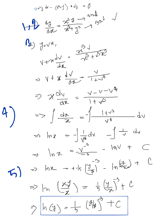
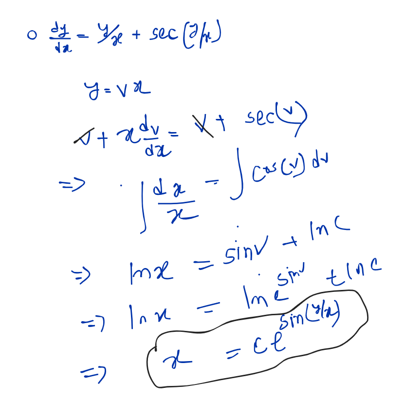
Step to Solve a Homogenous Differentiation Equation:

• Form the equation like $\frac{dy}{dx} = ...$

• $\frac{dy}{dx} = \frac{f(x,y)}{f(x,y)}$ Check the homogenous of the functions and degree individually, the functions must be homogenous and their degree must be same

• Put $y=vx$ int Step (1) equation and $\frac{dy}{dx} = v + x \frac{dv}{dx}$

• Apply Variable Separable Method

• Put $v = \frac{y}{x}$

Problems:

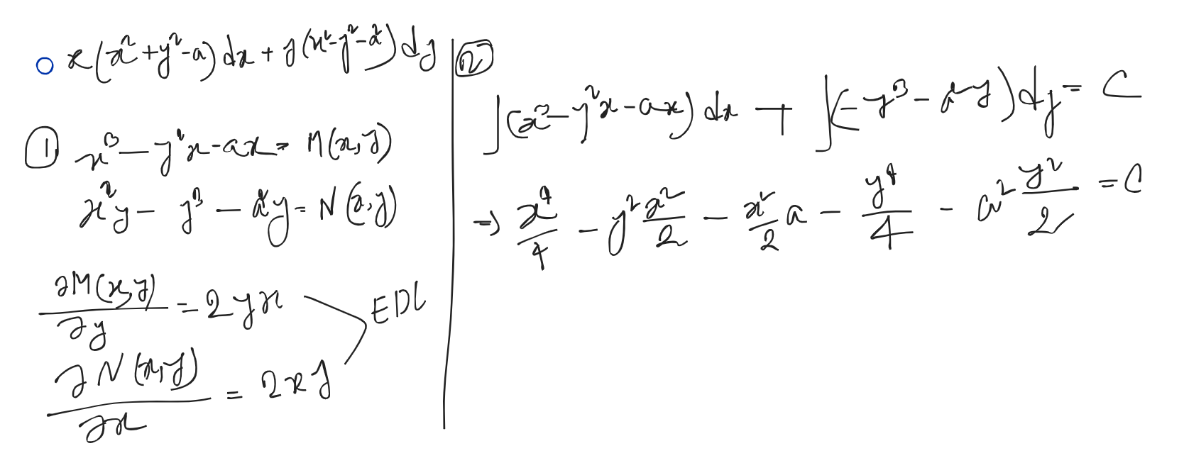
Exact Differentiation Equation:

Definition: $M(x,y) dx + N(x,y) dy = 0$ the equation will be Exact equation if $\frac{dM(x,y)}{dy} = \frac{dN(x,y)}{dx}$

[NB: y is constant when diff.w.r.t x and x is constant when diff.w.r.t y]

Steps:

• Check it a exact differentiation or not

• General Solution:

  $\int {M(x,y) dx \space [y \space is \space constant] } + \int{N(x,y) dy} \space [terms \space free \space from \space x ] = C$

Problems:

Reducible to Exact Differential Equation:

Steps:

Rule 1:

• Check the equation is exact or not, if not, go to next step

• ${\frac{\frac{dM}{dy} - \frac{dN}{dx}}{N}}$ and it is a function of only x or constant (not any single y) then go to next steps otherwise go to Rule 2

• Integrator factor IF = $e^{\int{\frac{\frac{dM}{dy} - \frac{dN}{dx}}{N}}}$

• Multiply the equation by the IF, then it is an exact equation now

• Follow the rules of EDE

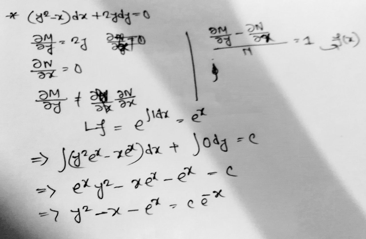
Correct Ans: $y^2 - x -1 = ce^{-x}$

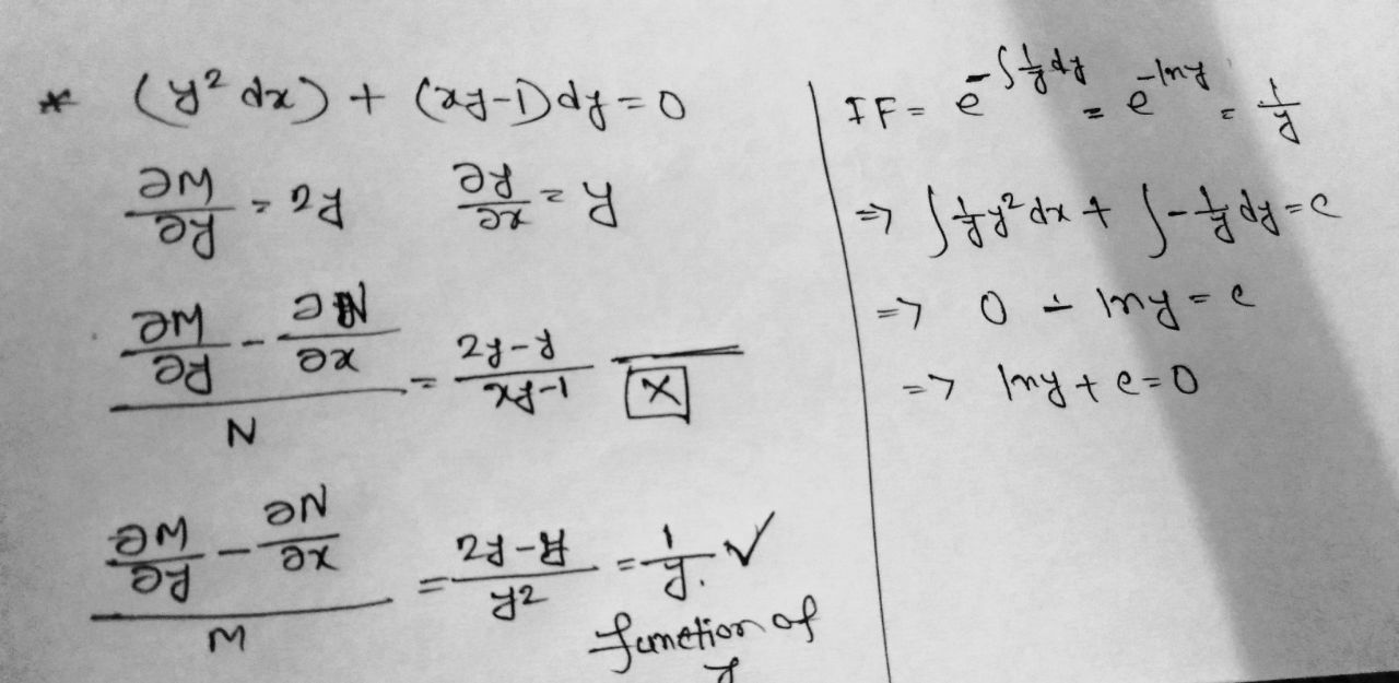
Rule 2:

• Check the equation is exact or not, if not, go to next step

• ${\frac{\frac{dM}{dy} - \frac{dN}{dx}}{M}}$ and it must be a function of only y or constant

• Integrator factor IF = $e^{- \int {\frac{\frac{dM}{dy} - \frac{dN}{dx}}{M}}}$ [There’s a minus sign]

• Multiply the equation by the IF, then it is an exact equation now

• Follow the rules of EDE

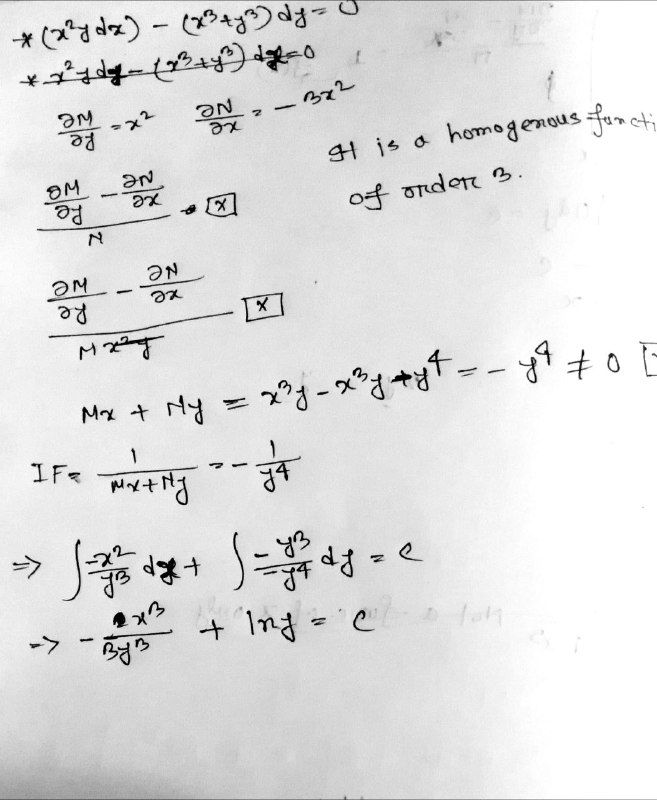
Rules 1: Homogenous Equation

• $Mdx + Ndy = 0$ is a homogenous equation and $Mx + Ny \not= 0$ then,

  IF = $\frac{1}{Mx+Ny}$

  Multiply by the IF , then the equation is now an exact equation.

• $Mdx + Ndy = 0$ is a homogenous equation and $Mx + Ny = 0$ then,

  IF = $\frac{1}{Mx-Ny}$

  Multiply by the IF , then the equation is now an exact equation.

Initial Value Problem:

First Order Equation:

$1) \frac{dy}{dx} = y \\ \space \\ y(0) = 3$

⇒ $\frac{dy}{y} = dx \\ or, \int\frac{dy}{y} = \int dx \\ or, lny = x + C \\ or, y = e^{x+c} \\ or, y = e^x . e^c \\ or, y = A e^x \\ \space \\ \space \\ \space \\ y(0) = 3 \\ or, Ae^0 = 3 \\ or ,A = 3 \\ \space \\ y = 3e^x$

Linear Differential Equation with Constant Coefficient:

$(\frac{d^ny}{dx^n} + P{_1}\frac{d^{n-1}x}{dy^{n-1}} + P{_2}\frac{d^{n-2}x}{dy^{n-2}} + .... P{_n})y = Q$

is a Linear Differential Equation if $P1, ....,Pn$ are the function of x or or constant.

If $P{_1},....,P{_n}$ are constant, then it is called Linear Differential Equation with Constant Coefficient.

If right hand side is zero or $Q=0$, then it is called Linear Homogenous Differential Equation.

$D = \frac{d}{dx}$

$D^2 = \frac{d^2}{dx^2}$

$.....$

$D^n = \frac{d^n}{dx^n}$

⇒ $(D^n + P{_1}D{_{n-1}} + ...+P{_n})y = Q$

1) If $Q=0$,

$y=CF$

Where, CF = Complementary Function

Complementary Function:

• Auxiliary Equation (AE)

  $(D^2 -7D+12)y = 0 \\ D^2 - 7D + 12 = 0 ...(i)$

  Where $(i)$ is an auxiliary equation

• Roots of AE

  $D^2 - 7D + 12 = 0 \\ or, m^2 - 7m + 12 =0 \\ m=3,4$

• Nature of Roots

  $Roots \space are \space real$

1) If $Q\not=0$

$Q = Q(x)$, a function of x

$y=CF + PI$

Where, CF = Complementary Function

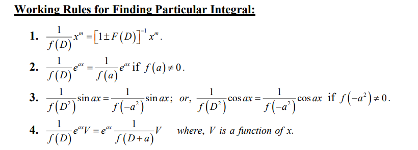
Particular Integral: (NOT AS SIR DID)

Type 1: $Q(x) = e^{ax}$ , $f(a) \not= 0$

CT:02

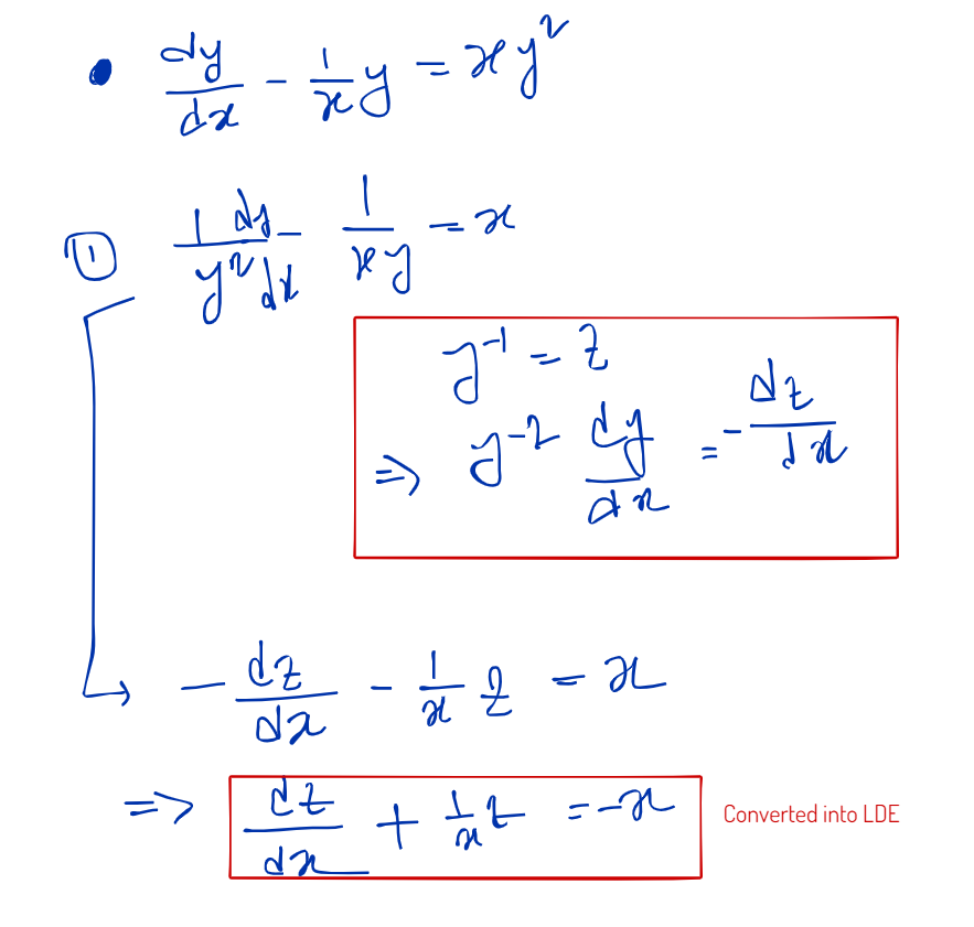
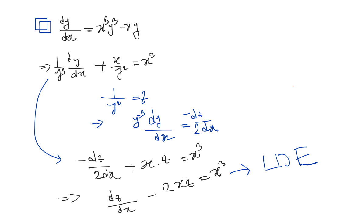
Bernoulli Differential Equation:

Definition: If P and Q are only functions of x or constants, then the differential equation of the form $\frac{𝑑𝑦}{𝑑𝑥}+𝑃𝑦 = 𝑄𝑦^𝑛$; $𝑛 ≠ 0$ is called Bernoulli’s equation

The Bernoulli Differentiation looks like,

$\frac{dy}{dx} + Py = Qy^n$

How to solve ? → Convert it to LDE. We have to vanish $y^n$ .

Steps:

• Dividing the equation by $y^n$ (besides Q)

• $z=y^m$ [besides P] and differentiate it w.r.t $x$

• Convert it to LDE

Problems:

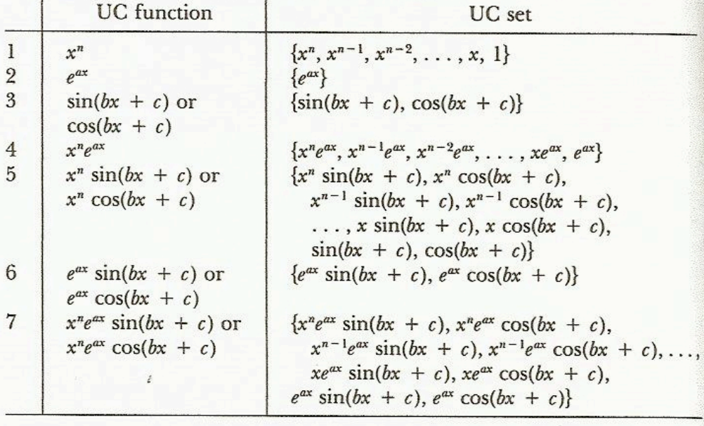
UC Method:

UC Function:

A function $f(x)$ is UC function, if it is either

• $x^n,$ where $n \ge 0$

• $e^{ax}$, where $a \not= 0$

• $sin(bx+c)$, $cos(bx+c)$, where $b \not=0$

• any function that is a finite product of two or more functions of these three types

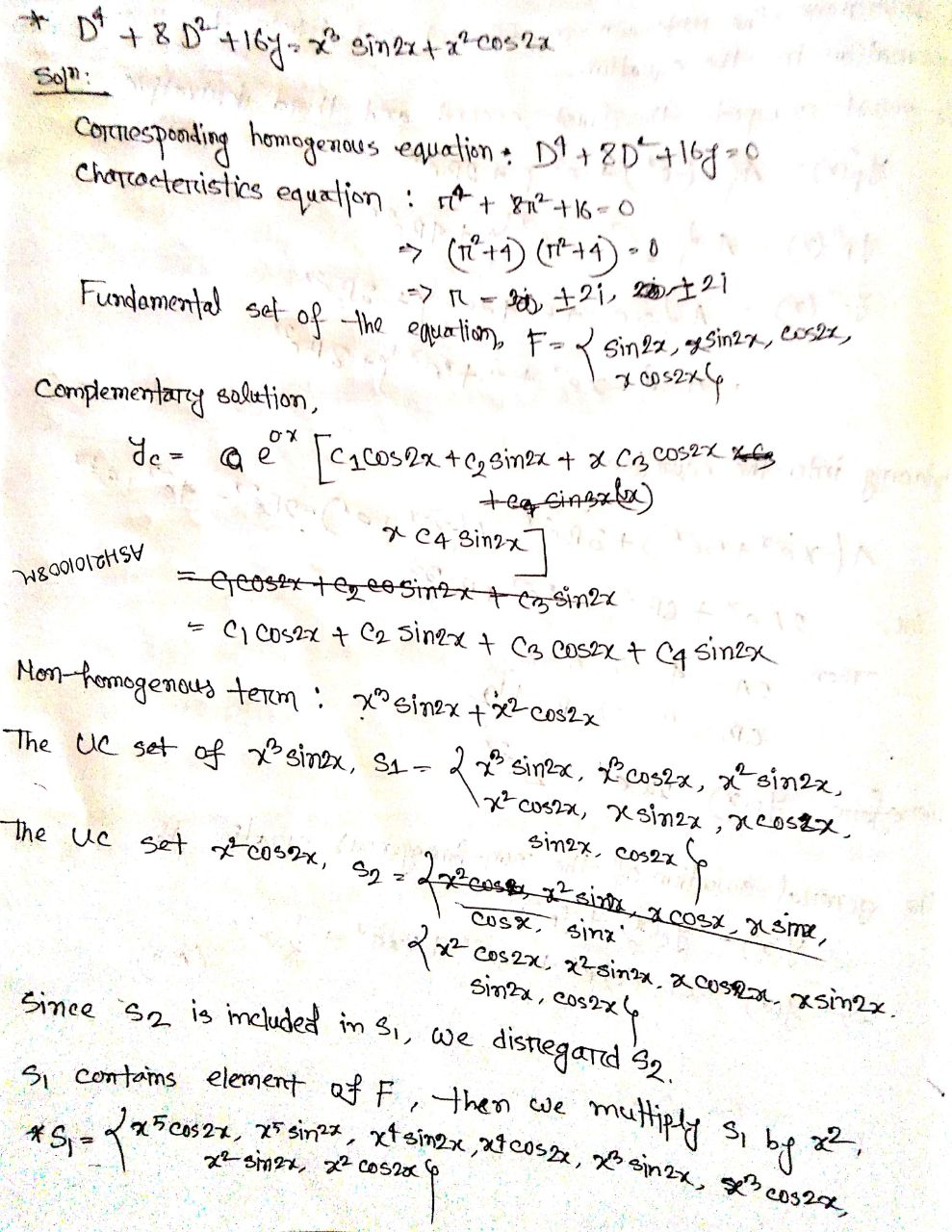
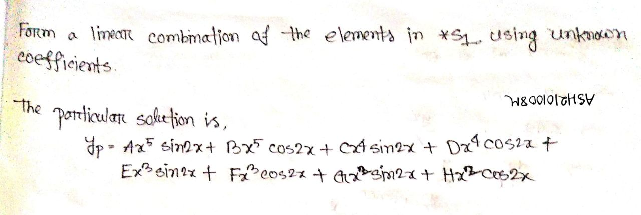
UC Set:

Definition: Given a UC function $f(x)$. We call UC set of $f(x)$, to the set of all UC functions consisting of $f(x)$ itself and all linearly independent functions of which the successive derivatives of $f(x)$ are either constant multiples or linear combinations.

Problems:

1)

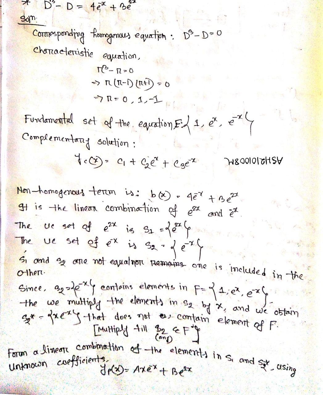
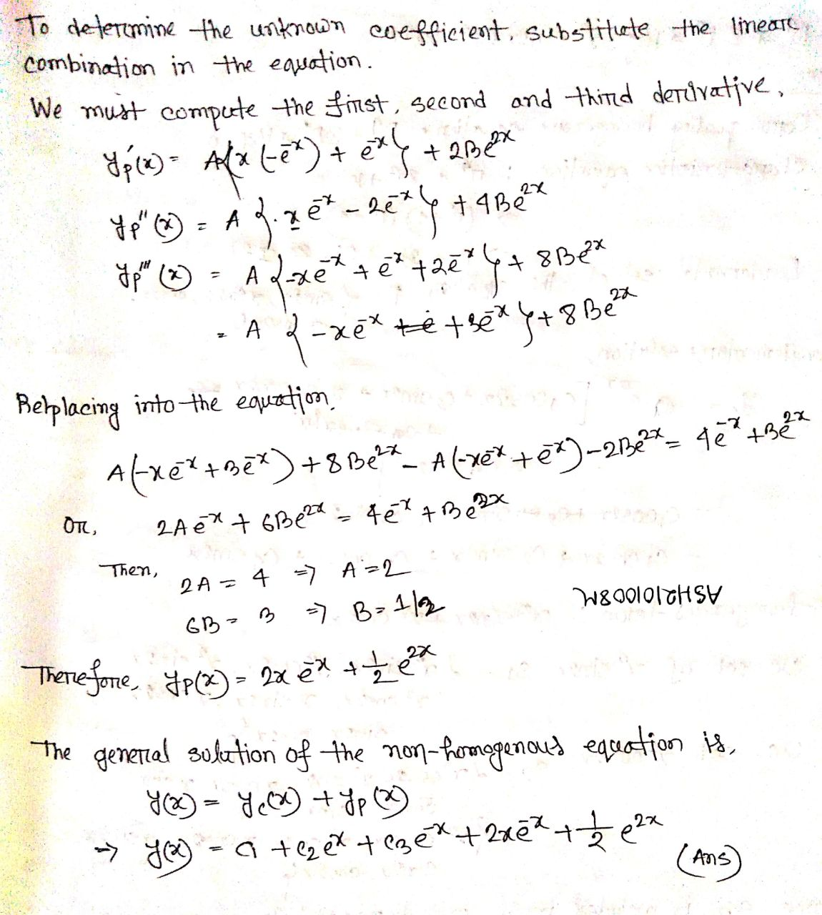
(comparing/equating left-hand side to right –hand side… 2A = 4 ….)

2)

Trajectories:

Trajectories: A curve which cuts every member of a given family of curves is called trajectories.

Orthogonal Trajectories: If a curve cuts every member of given family at right angles ($\alpha=90$), then it is called Orthogonal Trajectory.

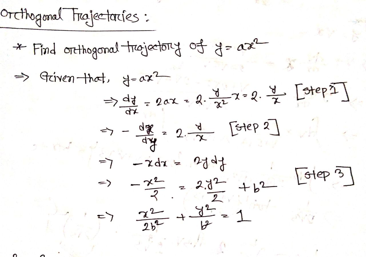
Working Rule:

• Differentiate the given equation of family of curve and eliminate parameter/constant

• Replace $\frac{dy}{dx}$ by $- \frac{dx}{dy}$

• Solve this new DE and get the orthogonal trajectory

Oblique Trajectory: A curve that intersects the curve of family at a constant angle $\alpha \not= 90$ is called Oblique Trajectories

Working Rule:

• Differentiate the given equation of family of curve and eliminate parameter/constant, denote it as $f(x,y)$

• $\frac{dy}{dx} = \frac{f(x,y) + tan\alpha}{1-f(x,y)tan\alpha}$ and solve the DE

Laplace Transform

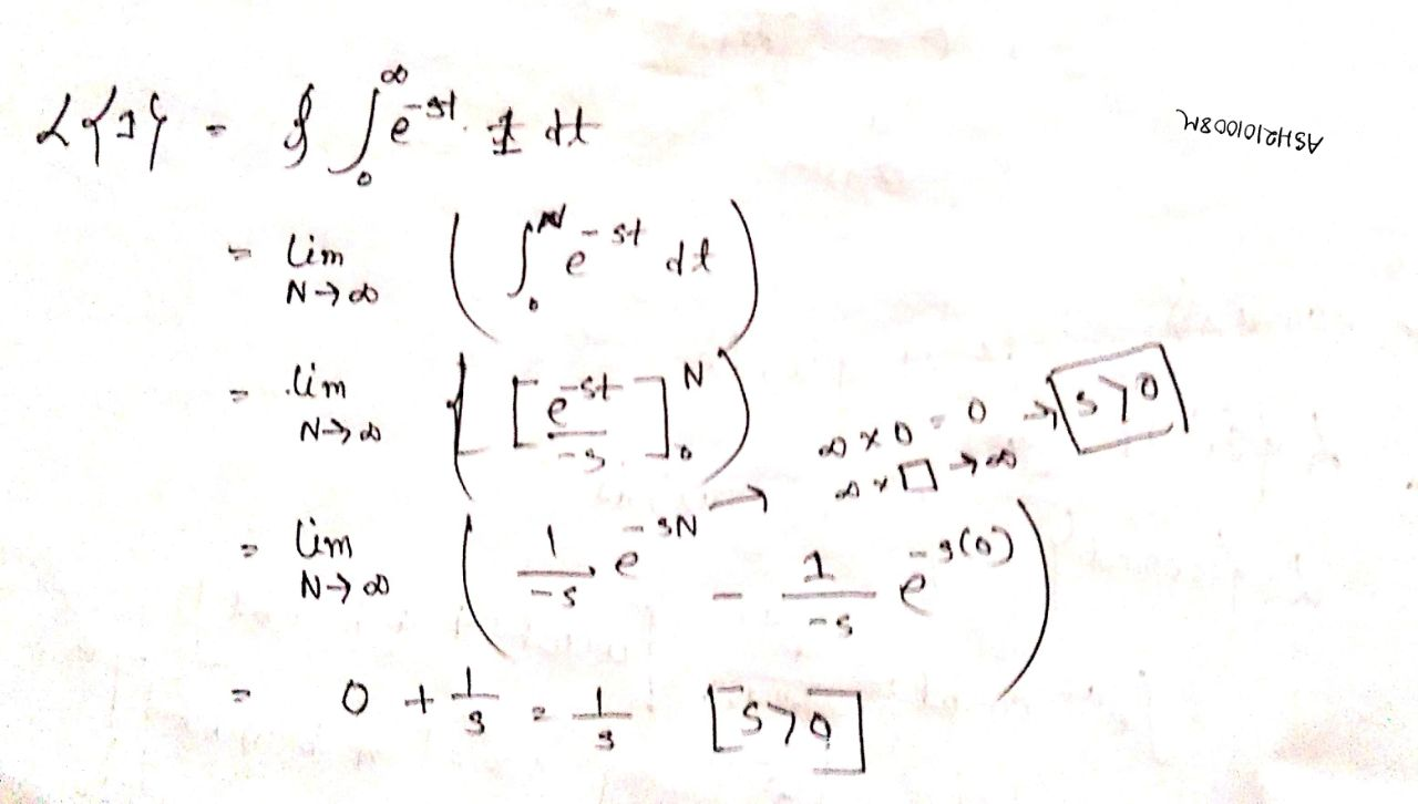
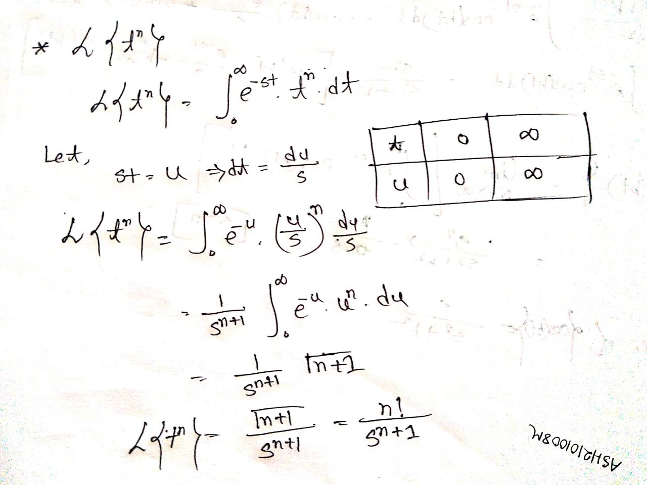
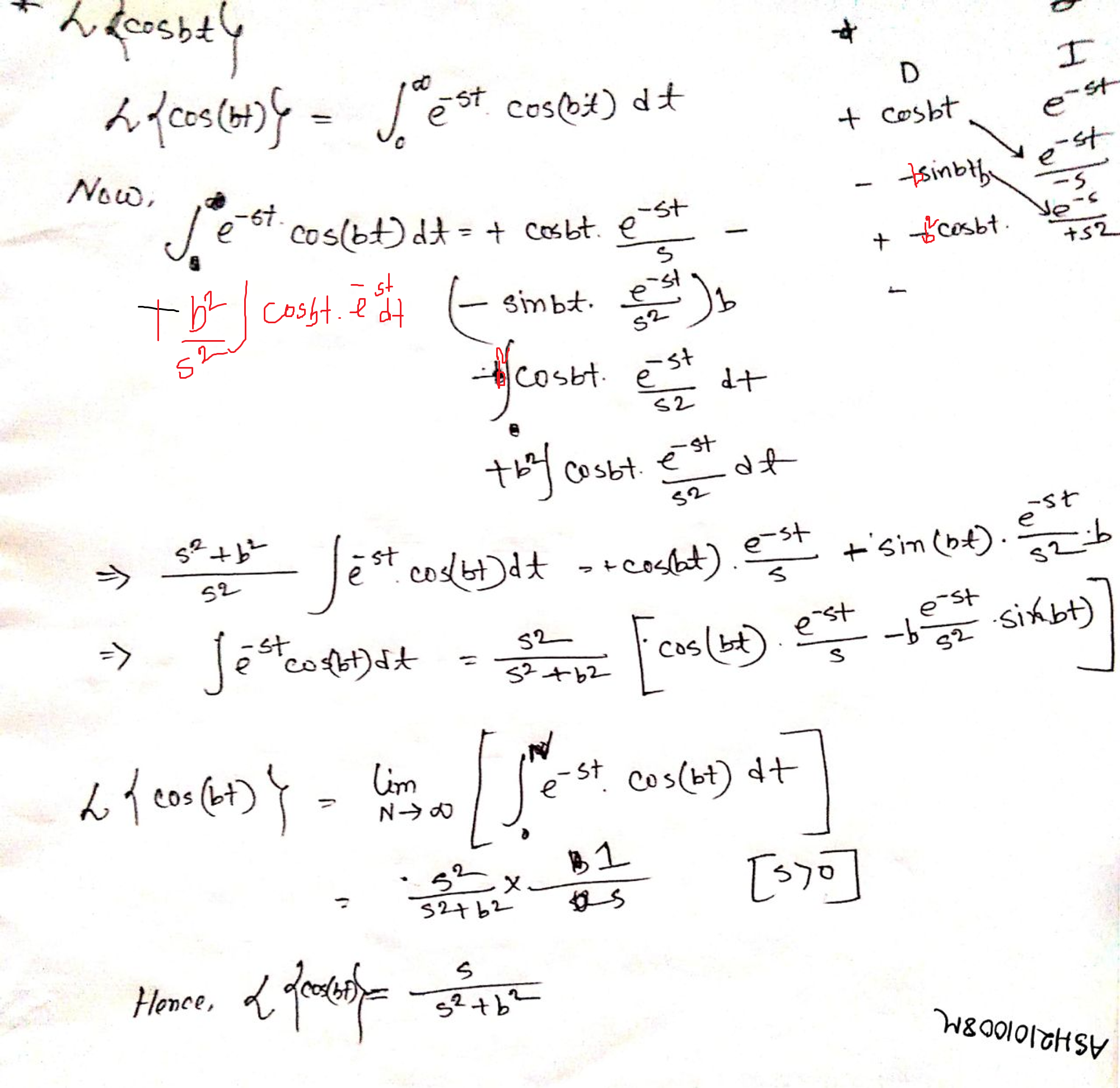
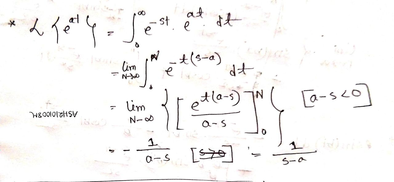
Definition: Let f(t) be a function of t defined for $0 \le t \lt \infin$

Then, Laplace transform of f(t) denoted by $\mathscr{L}\{ f(t) \}$ or $F(s)$, is defined by

$\mathscr{L}\{ f(t) \} = F(s) = \int_{0}^{\infin} e^{st} f(t) \,dt$

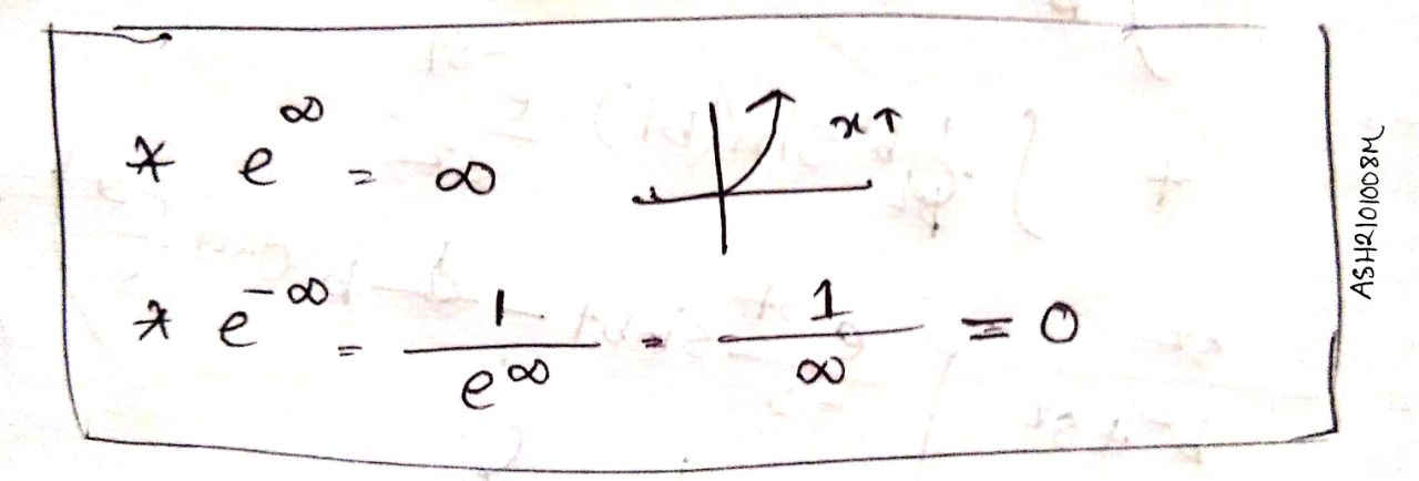
Reason why s > 0 || s < 0 || (a-s) < 0 →

Problems: